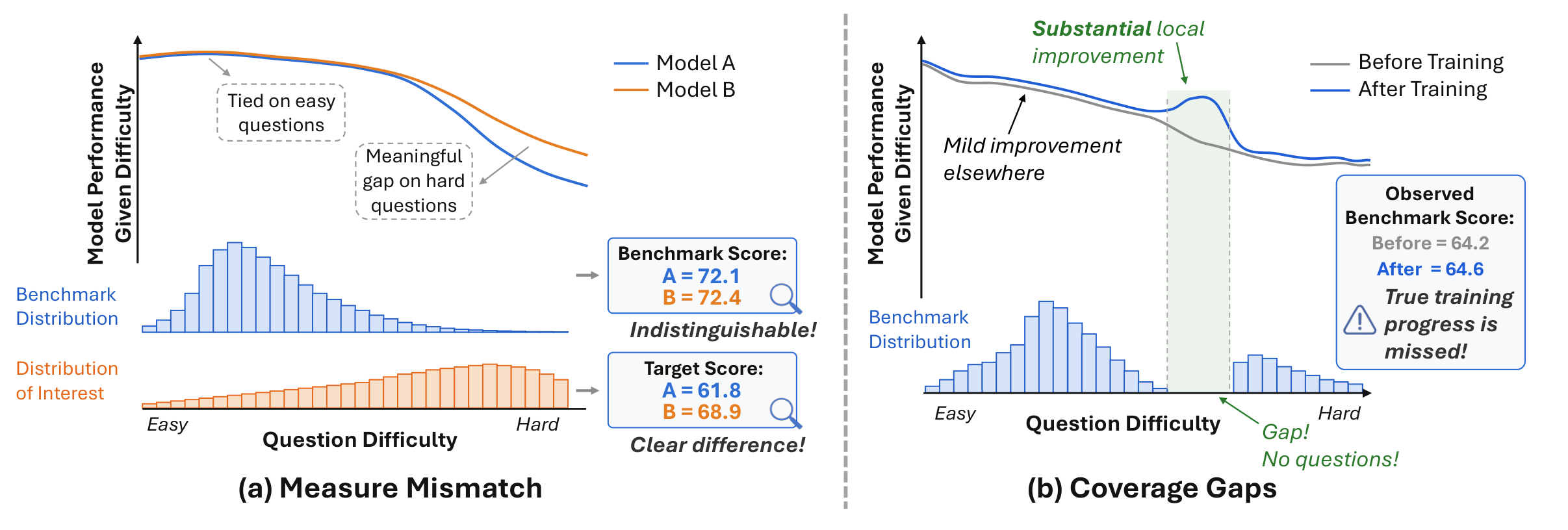
Benchmark evaluation looks simple: run models on a set of questions and average the results. But the conclusion depends not only on how well models perform, but also on how the benchmark's questions are distributed. Does a benchmark faithfully measure the model differences and training improvements we actually care about?
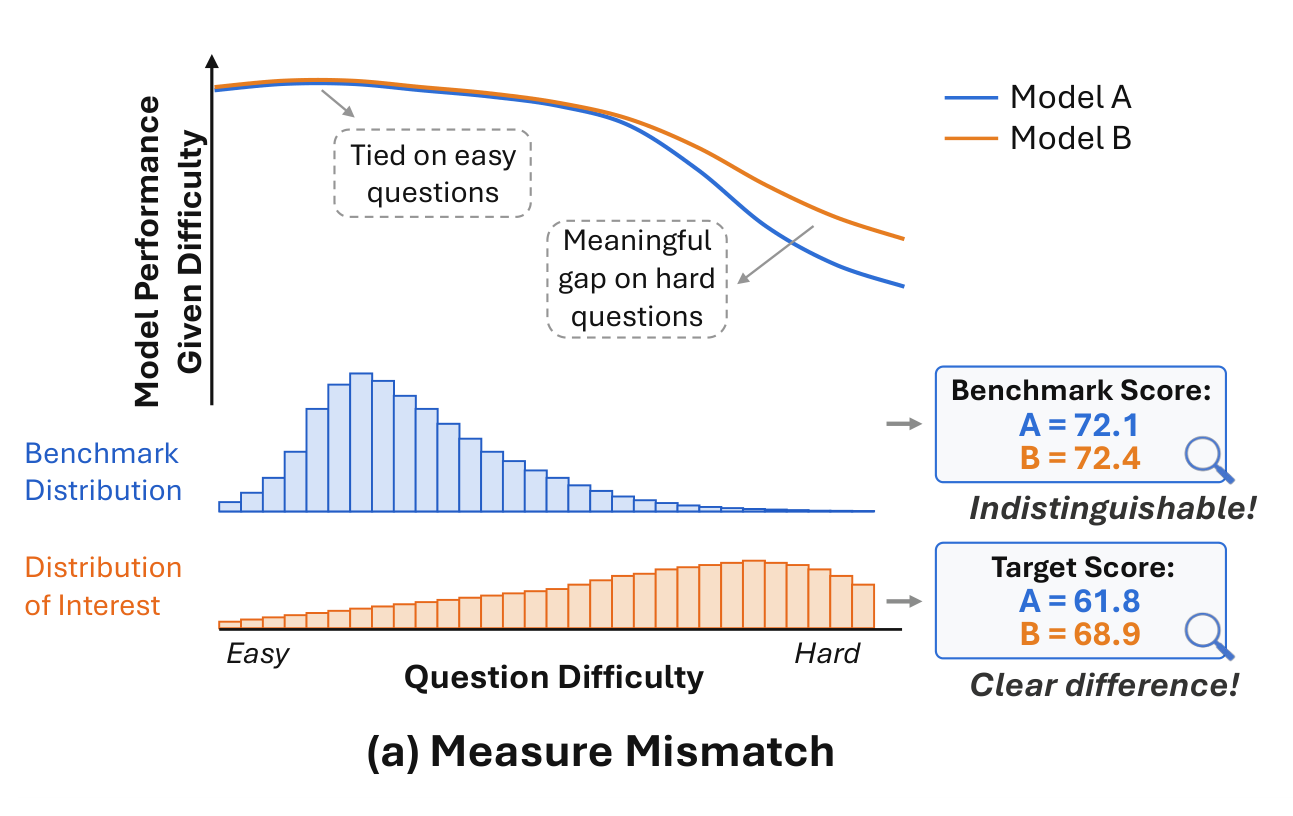
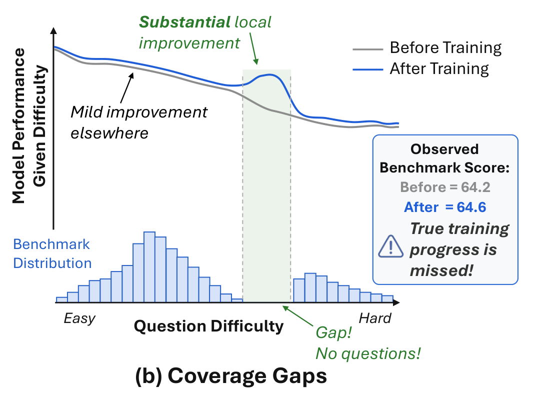
Two benchmark failure cases. In both panels, the curves show true model conditional performance as a function of question difficulty. (a) Measure Mismatch. The benchmark emphasizes easy questions, where the models perform similarly, while the difficulty distribution we care about places more weight on harder questions, where they differ substantially. Because the benchmark and the target distribution weight the difficulty axis differently, they lead to different conclusions for the same two models. (b) Coverage Gaps. A model actually improves substantially over a localized difficulty region. Because the benchmark has no questions in that region, this improvement is not reflected in the observed benchmark score, causing meaningful training progress to be missed. (Paper, Figure 1)
TL;DR
A benchmark induces an empirical measure over item difficulty: each question contributes equal mass at its difficulty level. This view exposes two fundamental problems.
Measure Mismatch
A benchmark’s empirical difficulty distribution may differ from the intended evaluation distribution, potentially distorting model comparisons.
Coverage Gaps
Uncovered intervals along the difficulty axis can prevent benchmarks from detecting meaningful localized model improvements.
A measure-based view of benchmarks
Place every benchmark item on a difficulty axis from 0 (easiest) to 1 (hardest). A model \(\theta\) is then described by its performance curve \(s_\theta(z)\): its expected performance, e.g., pass@1, on items of difficulty \(z\).
Benchmark measure
A benchmark \(B\) of \(n\) items with difficulties \(z_1,\dots,z_n\) puts equal mass \(1/n\) at each item: \[\nu_B=\frac1n\sum_{i=1}^n\delta_{z_i}.\]
Score as an integral
The usual average score is exactly an integral against this measure: \[S_B(\theta)=\frac1n\sum_{i=1}^n s_\theta(z_i)=\int s_\theta(z)\,d\nu_B(z).\]
Comparing two models works the same way: the benchmark reports \(D_B=\int\Delta\,d\nu_B\), where \(\Delta(z)=s_{\theta'}(z)-s_\theta(z)\) is their performance difference, so a leaderboard gap depends both on how the models differ and on where the benchmark places its items. What we actually want is \(D_\mu=\int\Delta\,d\mu\) under a target distribution \(\mu\) over difficulty that encodes the intended evaluation objective.
Two diagnostic metrics
Difficulty Distribution Mismatch
\[\mathrm{DDM}(B;\mu):=W_1(\nu_B,\mu)\]
The 1-Wasserstein distance: how much mass must be moved, and how far, to turn the benchmark's difficulty distribution into the target one.
The length of the largest interval on the difficulty axis that contains no benchmark item, counting the intervals next to 0 and 1 (\(z_{(0)}:=0\), \(z_{(n+1)}:=1\)).
What the theory guarantees
Theorem 2.1Distribution mismatch controls score distortion and rank stability
If the performance difference \(\Delta\) is \(L\)-Lipschitz, then
Consequently, if \(|D_\mu(\theta',\theta)|>L\,W_1(\nu_B,\mu)\), then \(\operatorname{sign}D_B(\theta',\theta)=\operatorname{sign}D_\mu(\theta',\theta)\): no rank flip can occur.
A small DDM keeps benchmark comparisons faithful to the target distribution.
Theorem 2.3Maximum gap as an exact asymptotic minimax detection boundary
Let \(s^-,s^+\) be the pre- and post-improvement performance curves. Fix \(\alpha\in(0,1)\) and \(a\in(0,1]\), and test \(H_0: s^-=s^+\) against \(H_1\): \(s^+(z)-s^-(z)\ge a\) for all \(z\) in some interval \(I\subset[0,1]\) with \(|I|=w\). Let \(\Pi^*_\alpha(B;w,a,k)\) be the minimax worst-case power of level-\(\alpha\) tests based on \(k\) repeated samples per item.
If \(w\le G(B)\), then \(\Pi^*_\alpha(B;w,a,k)=\alpha\) for every \(k\in\mathbb N\).
If \(w>G(B)\), then \(\lim_{k\to\infty}\Pi^*_\alpha(B;w,a,k)=1\).
An improvement no wider than the maximum gap can be invisible in the worst case, however many times the benchmark is re-run.
Diagnosing 25 popular benchmarks
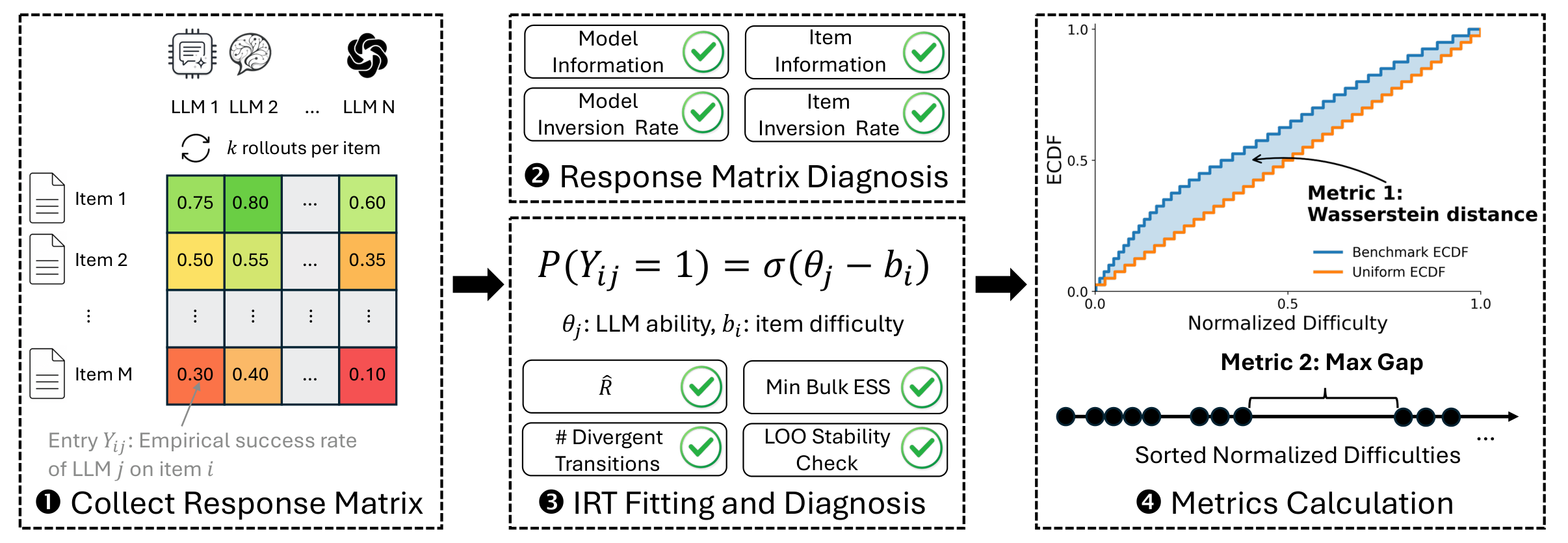
We analyze 25 widely used benchmarks spanning math, coding, agentic tasks, science, instruction following, logic, and medicine. Item difficulty is relative to model ability, so rather than using raw failure rates we estimate it with Item Response Theory (IRT). In the one-parameter logistic (1PL) model, model \(j\) solves item \(i\) with probability \(\Pr(Y_{ij}=1)=\sigma(\theta_j-b_i)\), where \(\theta_j\) is the model's ability and \(b_i\) the item's difficulty. Multiple-choice benchmarks add a chance-level guessing parameter.
Overview of our benchmark difficulty estimation and metric calculation pipeline. We collect empirical success rates from multiple LLMs on benchmark items, diagnose the response matrix, fit a 1PL IRT model to estimate item difficulties, perform post-fit IRT diagnostics, and compute two metrics over the normalized difficulty distribution. (Paper, Figure 2)
Model panel. For non-agentic benchmarks, 12 LLMs from 1.7B to 397B parameters, stratified across the Text Arena leaderboard, each with up to 32 rollouts per item. Agentic benchmarks use HAL results for 15–66 frontier closed-source LLMs.
Fitting and diagnostics. Bayesian inference via MCMC. A leave-one-out analysis supports the stability of the 12-model panel.
Metrics. Difficulties are normalized to \([0,1]\). DDM is measured against a same-size empirical uniform reference with points at \((i-\tfrac12)/n\), and gap metrics include the endpoint gaps.
25
benchmarks across 7 domains
10/25
have DDM ≥ 0.10
8/25
have Max Gap ≥ 0.10
9/25
have Top-5 Gap Sum ≥ 0.30
Interactive difficulty distribution explorer
Pick a benchmark to see the ECDF of its normalized item difficulties against the same-size uniform reference. The area between the two curves equals DDM, and the green bands mark the five largest adjacent gaps.
Table 1: Summary of proposed metrics across benchmarks. DDM denotes the 1-Wasserstein distance between the benchmark empirical difficulty distribution and a same-size empirical uniform distribution on [0, 1]. Max Gap is the largest gap between consecutive normalized difficulties, and Top-5 Sum is the sum of the five largest such gaps. # denotes the number of benchmark items. Lower is better for all three metrics. Highlighted entries mark comparatively large values for each metric: DDM ≥ 0.10, Max Gap ≥ 0.10, or Top-5 Sum ≥ 0.30. (Click a row to open it in the explorer.)
Benchmark
Domain
DDM
Max Gap
Top-5 Sum
#
Several benchmarks deviate strongly from the neutral uniform target. Their aggregate scores are more sensitive to over-represented difficulty regions and less sensitive to under-represented ones. Non-uniformity is not inherently a problem when it matches the intended evaluation objective. But when no such objective is specified, high-DDM leaderboard results reflect the benchmark's own difficulty weighting rather than a difficulty-neutral comparison, so users should check whether that weighting matches their use case.
Many benchmarks have large local coverage gaps. A training run may make meaningful progress inside an uncovered region while the aggregate score barely moves. AIME24 and AIME25, for example, have Top-5 Gap Sums close to 0.5 despite their widespread use for monitoring RLVR training. And this is not only a small-benchmark artifact: HumanEval (164 items) and BBH-5 objects (250 items) also show substantial gap metrics.
Difficulty-targeted gap filling
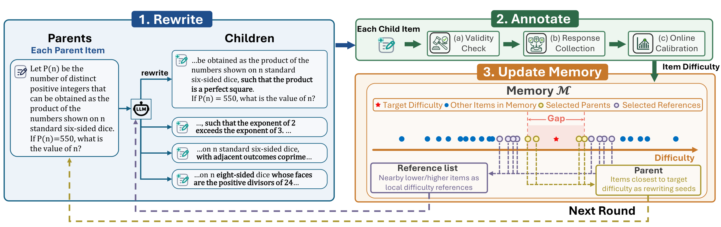
Diagnosis suggests an action: put new items where the benchmark has none. For an adjacent gap \([z_L,z_R]\) between two benchmark items, the goal is a valid new item whose difficulty is as close as possible to the midpoint \(z^\star=(z_L+z_R)/2\). The new item is added to the benchmark and replaces nothing. Rather than writing items from scratch, an LLM rewrites existing items, which serve as local difficulty references and keep the benchmark’s format and style.
Overview of the gap-filling method. Parent items are iteratively rewritten into child variants, the children’s difficulties are annotated, and the memory is updated to guide the next round of gap filling. (Paper, Figure 4)
Rewrite
Select relevant parent items and generate difficulty-targeted variants using the target difficulty and nearby reference items.
Annotate
Check candidate validity, collect model responses, and estimate the generated items’ difficulties through online IRT calibration.
Update Memory
Add annotated items to memory so subsequent generations can use better parents and difficulty references.
Results
We fill gaps in 8 representative benchmarks from different domains, targeting the three most pronounced gaps in each and inserting one item per gap. The rewriter is MiniMax-M2.7 (temperature 1.0). The search runs for at most 8 rounds, each with 4 parents × 4 children and a reference list of at most 16 nearby item–difficulty pairs, and stops early once an item is within 0.01 of the target. The baseline is a budget-matched best-of-N rewriter with uniformly sampled parents: it has the same rewrite budget and the same final selection rule, but no difficulty-aware retrieval, reference lists, or memory.
32.67%
average Top-3 Gap Sum reduction with our method (21.09%–38.88% per benchmark)
Top-3 Gap Sum Reduction (%) from the paper’s Table 2 (higher is better). The oracle sequentially inserts three items, each at the midpoint of the current largest gap.
Representative generated items
Each pair shows an original benchmark item (the ancestor) and the final item selected from its lineage, with the main change highlighted. Difficulties are normalized to [0,1], and the target is in parentheses. Rewrites can move difficulty in either direction.
AMC230.535 → 0.597
Original ancestor 0.535
For how many integers \(n\) does the expression \(\displaystyle\sqrt{\frac{\log(n^2)-(\log n)^2}{\log n-\htmlClass{hl}{3}}}\) represent a real number, where \(\log\) denotes the base-10 logarithm?
Generated item 0.597 (0.598)
Find the number of integer values of \(n\) such that \(\displaystyle\sqrt{\frac{\log(n^2)-(\log n)^2}{\log n-\htmlClass{hl}{1}}}\) represents a real number, where \(\log\) denotes the base-10 logarithm.
Gaokao2023en0.864 → 0.886
Original ancestor 0.864
On an \(8\times8\) chessboard, 6 black rooks and \(k\) white rooks are placed on different cells so that each rook only attacks rooks of the opposite color. Compute the maximum possible value of \(k\). (Two rooks attack each other if they are in the same row or column and no rooks are between them.)
Generated item 0.886 (0.885)
On a \(9\times9\) chessboard, 7 black rooks and \(k\) white rooks are placed on distinct squares so that each rook attacks only rooks of the opposite color. What is the maximum possible value of \(k\)? (Two rooks attack each other if they are in the same row or column and there is no rook between them.)
AIME250.750 → 0.674
Original ancestor 0.750
Alex divides a disk into four quadrants with two perpendicular diameters intersecting at the center of the disk. He draws 25 more line segments through the disk, each connecting two points at random on the perimeter in different quadrants. Find the expected number of regions into which these 27 line segments divide the disk.
Generated item 0.674 (0.671)
A circle has a diameter drawn, splitting it into two semicircular regions. Then 8 chords are drawn, each connecting a random point on the boundary in one semicircle to a random point on the boundary in the other semicircle. Assuming all points are chosen uniformly and independently, what is the expected number of regions into which the interior of the circle is divided?
Item text as shown in the paper's Table 13. All 24 gap-filling items, with answers, parents, targets, and annotated difficulties, are in new_item_records.csv in the code release.
Gap-filled benchmarks
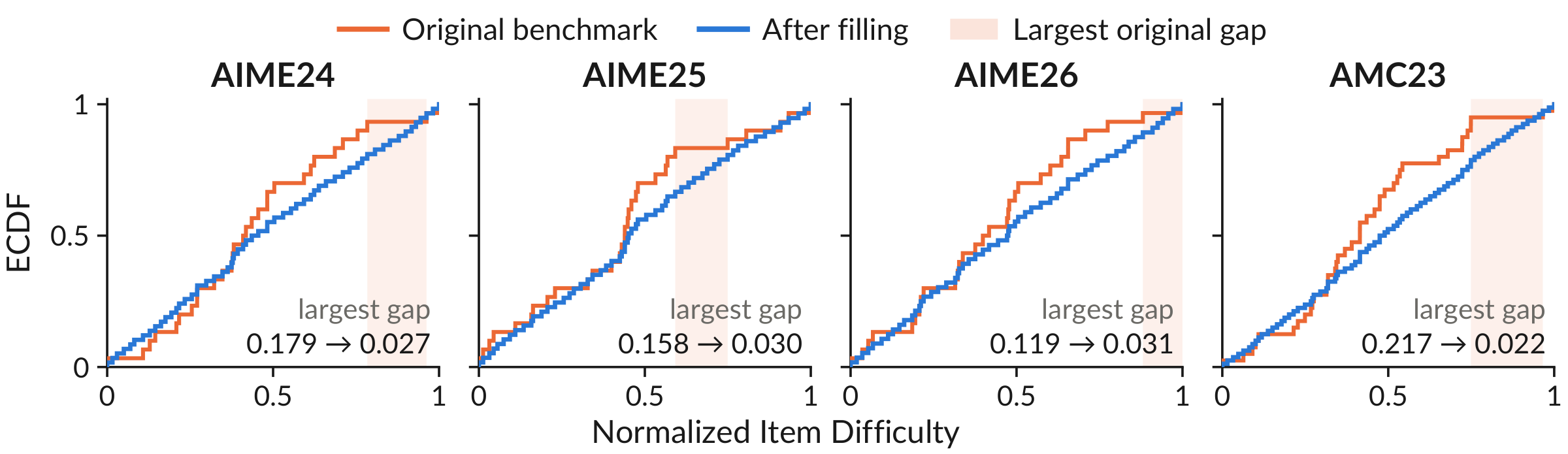
Difficulty distributions of AIME24, AIME25, AIME26, and AMC23 before and after difficulty-targeted gap filling. The shaded regions indicate the largest original coverage gaps.
We release augmented versions of these four math benchmarks. Each dataset contains the original benchmark questions followed by curated generated questions.
Augmented benchmark release: number of original, generated, and final questions.
@misc{sun2026benchmark,
  title  = {Your Benchmark Is an Empirical Measure Over Difficulty},
  author = {Sun, Yifan and Yu, Naicheng and Gong, Jiawen and Shen, Jingyan and Zhang, Huan},
  year   = {2026},
  note   = {Preprint}
}
Preprint citation. It will be updated with arXiv metadata once available.